High Dynamic Range Image Encodings
Greg Ward, Anyhere
Software
PDF version of this document (2.5 MBytes)
Introduction
We stand on the threshold of a new era in digital imaging, when image files will encode the color gamut and dynamic range of the original scene, rather than the limited subspace that can be conveniently displayed with 20 year-old monitor technology. In order to accomplish this goal, we need to agree upon a standard encoding for high dynamic range (HDR) image information. Paralleling conventional image formats, there are many HDR standards to choose from.
This article covers some of the history, capabilities, and future of existing and emerging standards for encoding HDR images. We focus here on the bit encodings for each pixel, as opposed to the file wrappers used to store entire images. This is to avoid confusing color space quantization and image compression, which are, to some extent, separable issues. We have plenty to talk about without getting into the details of discrete cosine transforms, wavelets, and entropy encoding. Specifically, we want to answer some basic questions about HDR color encodings and their uses.
What Is a Color Space, Exactly?
In very simple terms, the human visual system has three different types of color-sensing cells in the eye, each with different spectral sensitivities. (Actually, there are four types of retinal cells, but the “rods” do not seem to affect our sensation of color – only the “cones.” The cells are named after their basic shapes.) Monochromatic light, as from a laser, will stimulate these three cell types in proportion to their sensitivities at the source wavelength. Light with a wider spectral distribution will stimulate the cells in proportion to the convolution of the cell sensitivities and the light’s spectral distribution. However, since the eye only gets the integrated result, it cannot tell the difference between a continuous spectrum and one with monochromatic sources balanced to produce the same result. Because we have only three distinct spectral sensitivities, the eye can thus be fooled into thinking it is seeing any spectral distribution we wish to simulate by independently controlling only three color channels. This is called “color metamerism,” and is the basis of all color theory.
Thanks to metamerism, we can choose any three color “primaries,” and so long as our visual system sees them as distinct, we can stimulate the retina the same way it would be stimulated by any real spectrum simply by mixing these primaries in the appropriate amounts. This is the theory, but in practice, we must supply a negative amount of one or more primaries to reach some colors. To avoid such negative coefficients, the CIE designed the XYZ color space such that it could reach any visible color with strictly positive primary values. However, to accomplish this, they had to choose primaries that are more pure than the purest laser – these are called “imaginary primaries,” meaning that they cannot be realized with any physical device. So, while it is true that the human eye can be fooled into seeing many colors with only three fixed primaries, as a practical matter, it cannot be fooled into thinking it sees any color we like – certain colors will always be out of reach of any three real primaries. To reach all possible colors, we would have to have tunable lasers as our emitting sources. One day, we may have such a device, but until then, we will be dealing with restricted gamut color devices.
Figure 1 shows the perceptually uniform CIE (u´,v´) color diagram, with the positions of the CCIR-709 primaries. These primaries are a reasonable approximation to most CRT computer monitors, and officially define the boundaries of the standard sRGB color space. This triangular region therefore denotes the range of colors that may be represented by these primaries, i.e., the colors your eyes can be fooled into seeing. The colors outside this region, continuing to the borders of our diagram, cannot be represented on a typical monitor. More to the point, these “out-of-gamut” colors cannot be stored in a standard sRGB image file nor can they be printed or displayed using conventional output devices, so we are forced to show stand-in colors in this figure.
Figure 1. The CCIR-709 (sRGB) color gamut, shown within the CIE (u´,v´) color diagram.
The diagram in Figure 1 only shows two dimensions of what is a three-dimensional space. The third dimension, luminance, goes out of the page, and the color space (or gamut) is really a volume from which we have taken a slice. In the case of the sRGB color space, we have a six-sided polyhedron, often referred to as the “RGB color cube,” which is misleading since the sides are only equal in the encoding (0-255 thrice), and not very equal perceptually.
A color space is really two things. First, it is a set of formulas that define a relationship between a color vector or triplet, and some standard color space, usually CIE XYZ. This is most often given in the form of a 3´3 color transformation matrix, though there may be additional formulas if the space is non-linear. Second, a color space is a two-dimensional boundary on the volume defined by this vector, usually determined by the minimum and maximum value of each primary, which is called the color gamut. Optionally, the color space may have an associated quantization if it has an explicit binary representation. In the case of sRGB, there is a color matrix with non-linear gamma, and quantized limits for all three primaries.
What Is a Gamma Encoding?
In the case of a quantized color space, it is preferable for reasons of perceptual uniformity to establish a non-linear relationship between color values and intensity or luminance. By coincidence, the output of a CRT monitor has a non-linear relationship between voltage and intensity that follows a gamma law, which is a power relation with a specific constant (g) in the exponent:
In the above formula, output intensity is equal to some constant, K, times the input voltage or value, v, raised to a constant power, g. (If v is normalized to a 0-1 range, then K simply becomes the maximum output intensity, Imax.) Typical CRT devices follow a power relation corresponding to a g value between 2.4 and 2.8. The sRGB standard intentionally deviates from this value to a target g of 2.2, such that images get a slight contrast boost when displayed on a conventional CRT. Without going into any of the color appearance theory as to why this is desirable, let’s just say that people seem to prefer a slight contrast boost in their images. The important thing to remember is that most CRTs do not have a gamma of 2.2 – even if most standard color encodings do. In fact, the color encoding and the display curve are two very separate things, which have become mixed in most people’s minds because they follow the same basic formula, often mistakenly referred to as the “gamma correction curve.” We are not “correcting for gamma” when we encode primary values with a power relation – we are attempting to minimize visible quantization and noise over the target intensity range. (See Charles Poynton’s web pages on video encodings for a detailed explanation of gamma-related issues.)
Figure 2. Perception of quantization steps using a linear and a gamma encoding. Only 6 bits are used in this example encoding to make the banding more apparent, but the same effect takes place in smaller steps using 8 bits per primary.
Digital color encoding requires quantization, and errors are inevitable during this process. The point is to keep these errors below the visible threshold as much as possible. The eye has a non-linear response to intensity – at most adaptation levels, we perceive brightness roughly as the cube root of intensity. If we apply a linear quantization of color values, we see more steps in darker regions than we do in the brighter regions, as shown in Figure 2. Using a power law encoding with a g value of 2.2, we see a much more even distribution of quantization steps, though the behavior near black is still not ideal. (For this reason and others, some encodings such as sRGB add a short linear range of values near zero.) However, we must ask what happens when luminance values range over several thousand or even a million to one. Simply adding bits to a gamma encoding does not result in a good distribution of steps, because we can no longer assume that the viewer is adapted to a particular luminance level, and the relative quantization error tends towards infinity as the luminance tends towards zero.
What Is a Log Encoding?
To encompass a large range of values when the adaptation luminance is unknown, we really need an encoding with a constant or nearly constant relative error. A log encoding quantizes values using the following formula rather than the power law given earlier:
This formula assumes that the encoded value v is normalized between 0 and 1, and is quantized in uniform steps over this range. Adjacent values in this encoding thus differ by a constant factor, equal to:

where N is the number of steps in the quantization. This is in contrast to a gamma encoding, whose relative step size varies over its range, tending towards infinity at zero. The price we pay for constant steps is a minimum representable value, Imin, in addition to the maximum intensity we had before.
Figure 3. Relative error percentage plotted against log10 of image value for three encoding methods.
Another alternative closely related to the log encoding is a separate exponent and mantissa representation, better known as floating point. Floating point representations do not have perfectly equal step sizes, but follow a slight sawtooth pattern in their error envelope, as shown in Figure 3. To illustrate the quantization differences between gamma, log, and floating point encodings, we chose a bit size (12) and range (0.001 to 100) that could be reasonably covered by all three types. We chose a floating point representation with 4 bits in the exponent, 8 bits in the mantissa, and no sign bit since we are just looking at positive values. By denormalizing the mantissa at the bottom end of the range, we can also represent values between Imin and zero in a linear fashion, as we have done in this figure. By comparison, the error envelope of the log encoding is constant over the full range, while the gamma encoding error increases dramatically after just two orders of magnitude. Using a larger constant for g helps this situation somewhat, but ultimately, gamma encodings are not well-suited to full HDR imagery where the input and/or output ranges are unknown.
What Is a Scene Referred Standard?
Most image encodings fall into a class we call output referred standards, meaning they employ a color space corresponding to a particular output device, rather than the original scene they are meant to represent. The advantage of such a standard is that it does not require any manipulation prior to display on a targetted device, and it does not “waste” resources on colors that are out of this device gamut. Conversely, the disadvantage of such a standard is that it cannot represent colors that may be displayable on some other output device, or may be useful in image processing operations along the way.
A scene referred standard follows a different philosophy, which is to represent the original, captured scene values as closely as possible. Display on a particular output device then requires some method for mapping the pixels to the device’s gamut. This operation is referred to as tone mapping, and may be as simple as clamping RGB values to a 0-1 range, or something more sophisticated, like compressing the dynamic range or simulating human visual abilities and disabilities. The chief advantage gained by moving tone mapping to the image decoding and display stage is that we can produce correct output for any display device, now and in the future. Also, we have the freedom to apply complex image operations without suffering losses due to a presumed range of values.
The challenge of encoding a scene referred standard is finding an efficient representation that covers the full range of color values in which we are interested. This is precisely where HDR image encodings come into play.
What Are Some Applications of HDR Images?
Anywhere you would use a conventional image, you can use an HDR image instead by applying a tone mapping operation to get into the desired color space. The reverse is not true, because a conventional, output referred image cannot have its gamut extended to encompass a greater range – that information has been irretrievably lost. Therefore, HDR image applications are strictly a superset of conventional image applications, and suggest many new opportunities, which we have only begun to explore.
Below, we name just a few example applications that require HDR images as their input or as a critical part of their pipeline:
- Global illumination techniques (i.e., physically-based rendering)
- Mixed reality rendering (e.g., special effects for movies and commercials)
- Human vision simulation and psychophysics
- Reconnaissance and satellite imaging (i.e., remote sensing)
- Digital compositing for film
- Digital cinema
The list of applications is continuing to grow, and in the future, we expect digital photography to become almost exclusively HDR, as it was in the classic age of film and darkroom developing. (Color negatives are effectively an HDR representation of scene values, and photographic printing is the original tone-mapping operation.)
HDR Image Encoding Standards
The following list of HDR image standards is not meant to be comprehensive. Several other “deep pixel” standards that have been employed over the years, both in research and industry. However, most of these formats are not truly “high dynamic range,” in the sense that they represent only an order of magnitude or so beyond the basic 24-bit RGB encoding, and most of them represent exactly the same color gamut. For this discussion, we are interested in pixel encodings that extend over 4 orders of magnitude, and prefer those which also encompass the visible color gamut, rather than a subset constrained by existing red, green, and blue monitor phosphors. If they meet these requirements, and have a luminance step size below 1% and good color resolution, they will be able to encode any image with fidelity as close to perfect as human vision is capable of discerning. We restrict our discussion to this class of encodings, with one or two exceptions.
Pixar Log Encoding (TIFF)
Computer graphics researchers and professionals have been aware of the limitations of standard 24-bit RGB representations for decades. One of the first groups to arrive at a standard for HDR image encoding was the Computer Graphics Division of Lucasfilm, which branched off in the mid-80’s to become Pixar. Pixar’s immediate need for HDR was to preserve their rendered images on the way out to their own custom film recorder. As many people know, film is capable of recording much more dynamic range than can be displayed on a typical CRT – close to 4 orders of magnitude instead of the usual 2, and generally with a log response rather than a gamma curve. Logically, Pixar settled on a logarithmic encoding, which Loren Carpenter implemented as a “codec” (compressor-decompressor) within Sam Leffler’s TIFF library.
The format stored the usual three channels, one for each of red, green, and blue, but used an 11-bit log encoding for each, rather than the standard 8-bit gamma-based representation. Using this representation, Pixar was able to encode a dynamic range of roughly 3.6 orders of magnitude (3600:1) in 0.4% steps. A step of 1% in luminance is just on the threshold of being visible to the human eye.
This format was still employed internally at Pixar as recently as a few years ago, but we are not aware of any regular applications using it outside the company. Its dynamic range of 3.8 orders of magnitude is marginal for HDR work, and it is not well-known to the computer graphics community, as there has never been a publication about it other than the source code sitting in Leffler’s TIFF library. The lack of a negative range for the color primaries also means that the color gamut is restricted to lie within the triangle defined by the selected primary values.
Radiance RGBE Encoding (HDR)
In 1985, the author began development of the Radiance physically-based rendering system at the Lawrence Berkeley National Laboratory. Because the system was designed to compute photometric quantities, it seemed unacceptable to throw away this information when writing out an image, so we settled on a 4-byte representation where three 8-bit mantissas shared a common 8-bit exponent. Had we spent a little more time examining the Utah Raster Toolkit, we might have noticed therein Rod Bogart had written an “experimental” addition that followed precisely the same logic to arrive at an almost identical representation as ours. (Rod later went on to develop the EXR format at Industrial Light and Magic, which we will discuss in a moment.) In any case, the RGBE encoding was written up in an article in Jim Arvo’s Graphics Gems II, and distributed as part of the freely available Radiance system.
As the name implies, the Radiance RGBE format uses one byte for the red mantissa, one for the green, one for the blue, and one for a common exponent. The exponent is used as a scaling factor on the three linear mantissas, equal to 2 raised to the power of the exponent minus 128. The largest of the three components will have a mantissa value between 128 and 255, and the other two mantissas may be anywhere in the 0-255 range. The net result is a format that has an absolute accuracy of about 1%, covering a range of over 76 orders of magnitude.
Although RGBE is a big improvement over the standard RGB encoding, both in terms of precision and in terms of dynamic range, it has some important shortcomings. Firstly, the dynamic range is much more than anyone else could ever utilize as a color representation. The sun is about 108 cd/m2, and the underside of a rock on a moonless night is probably around 10-6 or so, leaving about 62 orders of useless magnitude. It would have been much better if the format had less range but better precision in the same number of bits. This would require abandoning the byte-wise format for something like a log encoding. Another problem is that any RGB representation restricted to a positive range, such as RGBE and Pixar’s Log format, cannot cover the visible gamut using any set of “real” primaries. Employing “imaginary” primaries, as in the CIE XYZ color system, can encode the visible gamut with positive values, but often at the expense of coding efficiency since many unreal colors will also be represented – similar to the useless dynamic range issue. Finally, the distribution of error is not perceptually uniform with this encoding. In particular, step sizes may become visible in saturated blue and magenta regions where the green mantissa drops below 20. These shortcomings led us to develop a much better format, described next.
SGI LogLuv (TIFF)
Working at SGI in 1997, the author set about correcting the mistakes made with RGBE, in hopes of providing an industry standard for HDR image encoding. This ultimately resulted in a LogLuv codec in Sam Leffler’s TIFF library. This encoding is based on visual perception, and designed such that the quantization steps match human contrast and color detection thresholds (a.k.a. “just noticeable differences”). The key advantage is that quanta in the encoding are held below the level that might result in visible differences on a “perfect” display system. Its design is similar in spirit to a YCC encoding, but with the limitations on color gamut and dynamic range removed. By separating the luminance and chrominance channels, and applying a log encoding to luminance, we arrive at a very efficient quantization of what humans are able to see. This encoding and its variants were described in the 1998 Color Imaging Conference paper, “Overcoming Gamut and Dynamic Range Limitations in Digital Images.”
There are actually three variants of this logarithmic encoding. The first pairs a 10-bit log luminance value together with a 14-bit CIE (u´,v´) lookup to squeeze everything into a standard-length 24-bit pixel. This was mainly done to prove a point, which is that following a perceptual model allows you to make much better use of the same number of bits. In this case, we were able to extend to the full visible gamut and 4.8 orders of magnitude of luminance in just imperceptible steps. The second variation uses 16 bits for a pure luminance encoding, allowing negative values and covering a dynamic range of 38 orders of magnitude in 0.3% steps, which are comfortably below the perceptible level. The third variation uses the same 16 bits for signed luminance, then adds 8 bits each for CIE u´ and v´ coordinates to encompass all the visible colors in 32 bits/pixel.
Although the LogLuv format has been adopted by a number of computer graphics researchers, and its incorporation in Leffler’s TIFF library means that a number of programs can read it even if they don’t know they can, it has not found the widespread use we had hoped. Part of this is people’s reluctance to deviate from their familiar RGB color space. Even something as simple as a 3´3 matrix to convert to and from the library’s CIE XYZ interface is confounding to many programmers. Another issue is simply awareness – unless one has key industry partners, it is difficult to get word out on a new format, no matter what its benefits might be. The follow-up article, written for the ACM Journal of Graphics Tools (vol. 3, no. 1), “LogLuv encoding for full-gamut, high-dynamic range images,” was an effort to stem these difficulties. We are still hopeful that this format will find wider use, as we have found it to work extremely well for HDR image encoding, ourselves. There is no more appropriate format for the archival storage of color images, at least until evolution provides an upgrade to human vision.
ILM OpenEXR (EXR)
In 2002, Industrial Light and Magic published C++ source code for reading and writing their OpenEXR image format, which has been used internally by the company for special effects rendering and compositing for a number of years. This format is a general-purpose wrapper for the 16-bit Half data type, which has also been adopted by both NVidia and ATI in their floating-point frame buffers. Authors of the OpenEXR library include Florian Kainz, Rod Bogart (of Utah RLE fame), Drew Hess, Josh Pines, and Christian Rouet. The Half data type is a logical contraction of the IEEE-754 floating point representation to 16 bits. It has also been called the “S5E10” format for “Sign plus 5 exponent plus 10 mantissa,” and this format has been floating around the computer graphics hardware developer network for some time. (OpenEXR also supports a standard IEEE 32-bit/component format, and a 24-bit/component format introduced by Pixar, which we will not discuss here due to their larger space requirements.)
Because it can represent negative primary values along with positive ones, the OpenEXR format covers the entire visible gamut and a range of about 10.7 orders of magnitude with a relative precision of 0.1%. Since humans can simultaneously see no more than 4 orders of magnitude, this makes OpenEXR a good candidate for archival image storage. Although the basic encoding is 48 bits/pixel as opposed to 32 for the LogLuv and RGBE formats, the additional precision is valuable when applying multiple blends and other operations where errors might accumulate. It would be nice if the encoding covered a larger dynamic range, but 10.7 orders is adequate for most purposes, so long as the exposure is not too extreme. The OpenEXR specification offers the additional benefit of extra channels, which may be used for alpha, depth, or spectral sampling. This sort of flexibility is critical for high-end compositing pipelines, and would have to be supported by some non-standard use of layers in a TIFF image.
We predict that the OpenEXR format will find widespread use in the computer graphics research community and special effects industry, as it has clear advantages for high quality image processing, and is supported directly by today’s high-end graphics cards. ILM is to be commended for offering their excellent library for license-free use, and given the complexity of the most common file variant, PIZ lossless wavelet compression, reimplementing EXR in a private library seems a formidable task.
Microsoft/HP scRGB Encoding
A new set of encodings for HDR image representation have been proposed by Microsoft and Hewlett-Packard, and accepted as an IEC standard (61966-2-2). The general format is called scRGB, formerly known as sRGB64. This standard grew out of the sRGB specification developed by Michael Stokes, Matthew Anderson, Srinivasan Chandrasekar, and Ricardo Motta, at HP and Microsoft. In essence, it is a logical extension of 24-bit sRGB to 16 linear bits per primary, or 12 bits per primary using a gamma encoding.
The scRGB standard is broken into two parts, one using 48 bits/pixel in an RGB encoding and the other employing 36 bits/pixel either as RGB or YCC. In the 48 bits/pixel substandard, scRGB specifies a linear ramp for each primary. Presumably, a linear ramp is employed to simplify graphics hardware and image-processing operations. However, a linear encoding spends most of its precision at the high end, where the eye can detect little difference in adjacent code values. Meanwhile, the low end is impoverished in such a way that the effective dynamic range of this format is only about 3.5 orders of magnitude – not really adequate from human perception standpoint, and too limited for light probes and HDR environment mapping. The standard does allow for negative primaries, which is an improvement over earlier RGB standards, but it makes wasteful use of this capability as much of the range is given to representing imaginary colors outside of the visible gamut, especially at the bottom end of the scale, where human color perception actually degrades. At the top end of its dynamic range, where people see colors more clearly, the gamut collapses in on itself again as primaries get clipped to the maximum representable value. This can be visualized on the colorspace animation page.
The second part of the scRGB standard offers a more sensible and compact 36 bits/pixel specification, which employs a standard gamma ramp with a linear subsection near zero. Although it uses 25% fewer bits, it has nearly as great a dynamic range as the 48-bit version, 3.2 orders as opposed to 3.5, and also allows negative primary values. It still suffers from a collapsing of its gamut at the top end and the unusable colors at the bottom, but it’s a better encoding overall. Even better than this scRGB-nl substandard is the scYCC-nl encoding, which benefits from a separate luminance channel and a color space that does not collapse quite as quickly at the top end. However, there is some strange behavior at peak luminance where the brightest representable value is not white, but follows a ring of partially saturated colors around white. This is because Cb and Cr contribute to the final luminance, so colored values (where Cb and Cr are non-zero) can be brighter than neutral ones. The net result is that colored light sources can become more saturated rather than less saturated during standard gamut clamping – fading to hot pink, for example. This situation is illustrated in Figure 4, below. This may also be seen on the colorspace animation page. In most situations, this would be an unexpected result, so care should be exercised when performing gamut mapping into scYCC-nl.
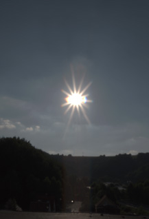
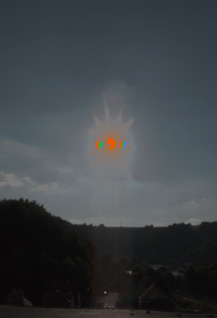
Figure 4. Gamut clamping anomalies using the scYCC-nl encoding. The first image shows a linear tone-mapping with clamping on the original HDR image of the sun. The second image shows the effect of simple clamping into an scYCC-nl gamut. Strange colorations result from the fact that the maximum representable luminances in scYCC-nl are not white.
It is unclear where the scRGB standard is headed at this point. Microsoft is promoting an undisclosed variant of this standard for use in digital cameras, graphics cards, and their Longhorn presentation engine, code named “Avalon” (October 2003 MS Developer’s Conference). In the case of digital cameras, the only competing high resolution standard is no standard at all – the so-called “RAW” image formats that are not only manufacturer-specific, but camera model-specific as well. This is a disaster from a user and software maintenance standpoint, and almost any data standard would be an improvement over the current situation. Modern graphics cards, on the other hand, have already adopted the Half floating point data type used in OpenEXR and the two leading manufacturers, NVidia and ATI, have designed their chips around it. There would seem to be little benefit in switching to a more limited integer standard such as scRGB at this point. As for image processing software, the only benefit over existing 48-bit integer RGB formats is the extended gamut, which comes at the expense of dynamic range. A 48-bit RGB pixel using a standard 2.2 gamma as found in conventional TIFF images holds at least 5.4 orders of magnitude, though applications like PhotoshopCS are not presently designed to use this range to best advantage. Image processing would probably be done in memory using 32-bit IEEE floats, and the scRGB standard would only be useful for file storage. However, scRGB and scRGB-nl/scYCC-nl hold less dynamic range than any of the other formats we have discussed for this purpose. We hope that the secret variant that Microsoft is promoting is a substantial improvement over the written IEC standard.
HDR Encoding Comparison
The following table summarizes the information given in the previous section. The first row entry in the chart shows 24-bit sRGB, which of course is not a high dynamic-range standard, but offered here as a baseline. The Bits/pixel value is for a tristimulus representation excluding alpha. The dynamic range is given as orders of magnitude, or the 10-based logarithm of the maximum representable value over the minimum value. The actual maximum and minimum are in parentheses. Dynamic range is difficult to pin down for non-logarithmic encodings such as scRGB, because the relative error is not constant throughout the range. We have selected 5% as the cut-off at the low end, when steps are considered too large to be included in the “useful” range. This is on the generous side, since viewers can detect luminance changes as small as 2%, but given that these errors usually occur in the darkest regions of the image, they may go unnoticed even at 5%. Non-logarithmic encodings are listed with “Variable” as their step size for this reason. Related formats with identical sizes and ranges are given together in the same row.
|
Encoding |
Covers Gamut |
Bits / pixel |
Dynamic Range |
Quant. Step |
|
sRGB |
No |
24 |
1.6 (1.0:0.025) |
Variable |
|
Pixar Log |
No |
33 |
3.8 (25.0:0.004) |
0.4% |
|
RGBE XYZE |
No Yes |
32 |
76 (1038:10-38) |
1% |
|
LogLuv 24 |
Yes |
24 |
4.8 (15.9:0.00025) |
1.1% |
|
LogLuv 32 |
Yes |
32 |
38 (1019:10-20) |
0.3% |
|
EXR |
Yes |
48 |
10.7 (65000:0.0000012) |
0.1% |
|
scRGB |
Yes |
48 |
3.5 (7.5:0.0023) |
Variable |
|
scRGB-nl scYCC-nl |
Yes Yes |
36 |
3.2 (6.2:0.0039) |
Variable |
Table 1. HDR encoding comparison chart.
As we can see from Table 1, RGBE and XYZE are the winners in terms of having the most dynamic range in the fewest bits, and the XYZE encoding even covers the visible gamut. However, 76 orders of magnitude is so far beyond the useful range, that we have chosen to show XYZE as an outlier on our plog (Figure 5).
Figure 5. Cost (bits/pixel) vs. benefit (dynamic range) of full-gamut formats.
Figure 5 shows quite clearly the benefits of log and floating point representations over linear or gamma encodings. In 24 bits, the LogLuv format holds more dynamic range than the 36-bit scRGB-nl format, which uses a gamma encoding, and even the 48-bit scRGB linear encoding, which occupies twice the number of bits. In 32 bits, the LogLuv encoding holds 10 times the dynamic range of either of these formats. The EXR encoding holds 3 times the range of scRGB encoding in the same 48 bits, with much higher precision than any of the other formats in our comparison.
Image Results
What difference does any of this make to actual images? To find out, we collected a set of HDR images from various sources in different formats and set about converting from one format to another to see what sorts of errors were introduced by the encodings. We took images from three sources: captured exposure sequences combined directly into 96-bit/pixel floating-point TIFF, Radiance-rendered images in RGBE format, other people’s captures in RGBE, and ILM-supplied captures in EXR format. In each case, we wrote out the image in a competing format and read it back, then did a pixel-by-pixel comparison. Comparing images visually is problematic, since high dynamic range displays are not currently available. The best we can do is run up and down locally with a linear tone-mapping, comparing the original and re-encoded images.
To be objective, we would also prefer a numerical comparison to a visual one. CIE ∆E* is a popular metric for quantifying color differences, but here again we run into difficulties when confronted with HDR input. Specifically, the CIE metric assumes a global white adaptation value, which makes sense for a paper task, but not for a scene where the brightest to the darkest regions may span a dynamic range of 10000:1. Relative to the brightest region in many of our images, the rest of the pixels would register as “a similar shade of black” as far as CIE 1994 is concerned. To cope with this problem, we decided to apply a “local reference white” in our comparisons, defined as the brightest pixel within 50 pixels of our current test position. The luminance of this brightest pixel, together with a global white point (chromaticity) for our image, is employed as the “reference white” in the CIE 1994 formula. This is not a perfect solution, and one could argue about the appropriate distance for choosing such a maximum, or if this is a valid approach at all, but it gave us what we were after, which was a measure of color differences between HDR images that roughly correlates with what we can see when we tone-map the regions locally.
Another problem we ran up against was optimizing the dynamic range for the desired comparison format. Especially for the LogLuv24 and scRGB-nl formats, the limited dynamic range available meant we needed to scale the original image to minimize losses at the top and bottom ends. Rather than coming up with a different scale factor optimized to the range of each format, we settled on one scale factor for each original image based on the most constrained destination, scRGB-nl. To find each factor, we examined the original image histogram and determined the scale factor that would deliver the largest population of pixels within the 6.2:0.0039 range of scRGB-nl. This factor was then applied to every format conversion for that image, simplifying our difference measurements. We expect this policy made the LogLuv24 results look worse than they should have, but did not adversely affect results from any other encodings.
To demonstrate how these comparisons work and why they are necessary, let’s start with an example. Figure 6a shows the familiar Memorial Church, tone-mapped to fit within a standard sRGB range. Figure 6b shows the same image passed through the 24-bit LogLuv encoding, which is not able to contain all of the original image’s dynamic range. However, the degradation is difficult to see here, because we had to compress the whole range into a much smaller destination space, 24-bit sRGB. To actually observe the effect of the LogLuv24 encoding, we must zoom into the brightest region of the image, the stained glass windows, and remap locally using a linear operator. This comparison is shown in Figure 7.
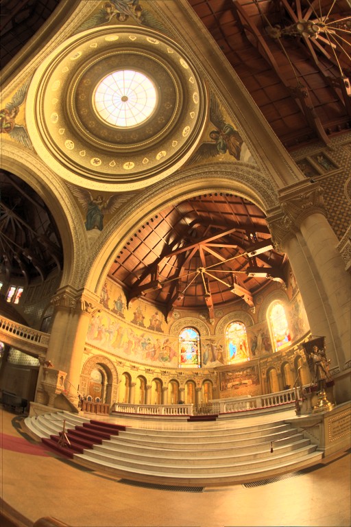

Figure 6. The Stanford Memorial Church. (Image courtesy Paul Debevec.) The first image is the original, tone-mapped into a printable range. The second image has been passed through the 24-bit LogLuv encoding prior to tone-mapping.
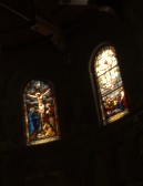

Figure 7. A close-up of the brightest region of the image with a linear tone-mapping. The original is shown on the left, and the subimage on the right has been passed through the 24-bit LogLuv encoding. Here we can see the losses incurred by exceeding the dynamic range of this encoding.
Through consistent application of our numerical difference metric, we can more easily identify problem areas. Figure 8 shows the difference metric comparing the original image with the version that has been passed through the 24-bit LogLuv encoding. This false color image highlights the errors in the window quite clearly, without the need for multiple scales and visual comparisons. The values corresponding to the color scale of the image are shown in the legend to the left. A ∆E* value of 1 corresponds to the human detection threshold for colors that are immediately adjacent to each other. A ∆E* value of 2 is generally considered visible for adjacent color patches, and ∆E* values of 5 or greater may be discerned without difficulty in side-by-side images. As we can see, the brightest window in this image contains ∆E* values greater than 12, indicated the differences are highly visible.
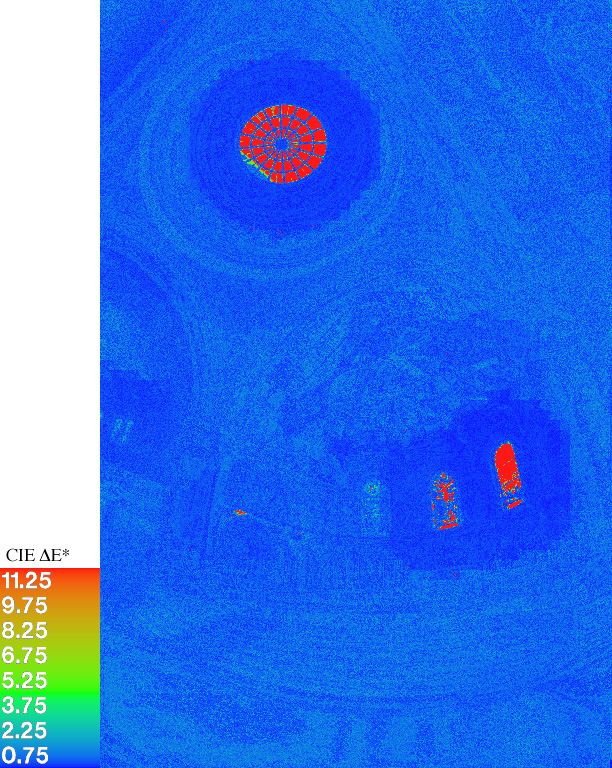
Figure 8. The modified 1994 CIE ∆E* metric showing the expected visible differences due to the 24-bit LogLuv encoding.
Figures 9 and 10 show the difference metrics and corresponding close-ups for the 32-bit LogLuv and 48-bit scRGB encodings, respectively.


Figure 9. The Memorial Church image loses very little passing through the 32-bit LogLuv encoding, as can be seen in the color difference analysis and in the detail on the right. (The false color scale is the same in all images.)
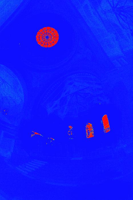

Figure 10. As expected from its limited dynamic range, the 48-bit scRGB pixel format suffers significant losses in its attempt to encode the Memorial Church image. The detail on the right shows just how little of the original dynamic range has been preserved by this encoding.
We have performed similar analyses on a total of 33 original images using 8 different HDR encodings. These images are linked to the originals page, which is in turn linked with the encoding difference pages. Although it might be instructive, it would be tedious to go through all of these images and compare the results visually, running up and down the range of possible exposures in each encoding. Even relying on our false color representations of color differences, we still have 264 before/after comparison images to examine. One useful way of condensing this information for a particular image is to plot the percentile of pixels above a particular CIE ∆E* value for each encoding. This set of curves is shown in Figure 11 for the Memorial Church image.
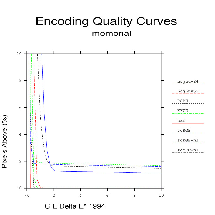
Figure 11. A plot showing the percentage of pixels above a particular ∆E* for each encoding of the Memorial Church image.
The ideal encoding behavior would be a steep descent that reached a very small percentile for anything above 2 on the CIE ∆E* axis. Indeed, this behavior is demonstrated by the EXR format in all of our example images, making it the clear winner in terms of color fidelity. This is not surprising, since the EXR format uses 48 bits/pixel and has smaller step sizes over its usable range than all the rest. The same cannot be said for the 48-bit scRGB format, which performed poorly in our comparisons – worse even than the lightweight 24-bit/pixel LogLuv encoding in terms of perceivable differences.
Results Summary
For our results summary in Table 2, we report a pair of values derived from our color difference metrics that we feel give a fair measure of how well a particular encoding performed on a particular HDR image. These are the percentile quantities taken from our plots for the percentage of pixels above two selected ∆E* values: ∆E*=2 and ∆E*=5. These correspond to the levels at which differences are detectable under ideal conditions and noticeable in side-by-side images, respectively.
Let’s look at the first row of our results summary in Table 2. For the 24-bit LogLuv encoding, this says that 6.92% of the Apartment image pixels have a ∆E* of 2 or greater, meaning that one could (under ideal circumstances) distinguish these pixels from their original values. This may or may not be significant, depending on how critical your application is. If small color differences are acceptable, we may not care about the lower threshold, because one would not be able to tell the pixels apart unless they were flashed one on top of the other. However, the table also indicates that 0.31% of the pixels have a ∆E* of 5 or greater, which means they would be visibly different in side-by-side images. This is a more important value; however, unless these pixels are all bunched together in some important part of the image, they are likely to escape notice because they represent such a small fraction of the total. In general, it is time to worry when more than 2% of the pixels have a ∆E* of 5 or greater, meaning that a noticeable fraction of the image has colors that are visibly different from the original. These entries are highlighted in magenta in our table. For critical work, we might also be concerned when the ∆E*is above 2 over more than 5% of the image, and we have highlighted these entries in yellow.
|
Image |
LogLuv24 |
LogLuv32 |
RGBE |
XYZE |
EXR |
scRGB |
scRGB-nl |
scYCC-nl |
|
6.92% |
0.00% |
0.00% |
0.00% |
0.00% |
1.21% |
5.14% |
2.63% |
|
|
3.35% |
0.00% |
0.00% |
0.00% |
0.00% |
0.27% |
0.31% |
0.30% |
|
|
5.95% |
1.05% |
1.56% |
0.81% |
0.00% |
8.68% |
9.92% |
8.26% |
|
|
0.74% |
0.00% |
0.00% |
0.00% |
0.00% |
0.72% |
0.99% |
0.73% |
|
|
1.56% |
0.00% |
0.00% |
0.00% |
0.00% |
0.08% |
0.09% |
0.06% |
|
|
2.54% |
0.00% |
0.00% |
0.00% |
0.00% |
0.12% |
0.26% |
0.22% |
|
|
4.19% |
0.00% |
0.00% |
0.00% |
0.00% |
0.11% |
0.15% |
0.19% |
|
|
4.47% |
0.00% |
0.00% |
0.00% |
0.00% |
0.00% |
0.01% |
0.09% |
|
|
11.14% |
0.00% |
0.00% |
0.00% |
0.00% |
0.32% |
0.33% |
0.37% |
|
|
2.32% |
0.00% |
0.00% |
0.00% |
0.00% |
0.27% |
0.49% |
0.39% |
|
|
9.97% |
0.00% |
0.00% |
0.00% |
0.00% |
0.97% |
1.06% |
1.00% |
|
|
2.16% |
0.00% |
0.05% |
0.02% |
0.00% |
4.89% |
5.79% |
16.30% |
|
|
0.74% |
0.01% |
0.01% |
0.01% |
0.00% |
6.42% |
9.21% |
3.03% |
|
|
2.02% |
0.00% |
0.00% |
0.00% |
0.00% |
0.09% |
0.11% |
0.10% |
|
|
2.61% |
0.00% |
0.01% |
0.01% |
0.00% |
1.51% |
1.72% |
1.58% |
|
|
0.64% |
0.00% |
0.02% |
0.02% |
0.00% |
2.64% |
3.80% |
2.40% |
|
|
5.06% |
0.00% |
0.00% |
0.00% |
0.00% |
0.00% |
2.70% |
0.00% |
|
|
1.31% |
0.00% |
0.00% |
0.00% |
0.00% |
1.76% |
1.85% |
1.65% |
|
|
1.66% |
0.00% |
0.01% |
0.00% |
0.00% |
2.10% |
2.35% |
1.95% |
|
|
13.76% |
0.00% |
0.00% |
0.00% |
0.00% |
0.01% |
0.02% |
0.05% |
|
|
6.53% |
0.00% |
0.00% |
0.02% |
0.00% |
0.19% |
0.72% |
0.72% |
|
|
1.51% |
0.02% |
0.26% |
0.17% |
0.00% |
0.23% |
0.25% |
0.08% |
|
|
3.85% |
0.00% |
0.00% |
0.00% |
0.00% |
1.71% |
1.93% |
1.91% |
|
|
3.18% |
0.00% |
0.00% |
0.00% |
0.00% |
0.05% |
0.57% |
0.00% |
|
|
1.72% |
0.00% |
0.00% |
0.00% |
0.00% |
0.08% |
0.09% |
0.15% |
|
|
4.89% |
0.00% |
0.00% |
0.00% |
0.00% |
0.76% |
0.80% |
0.81% |
|
|
12.05% |
0.00% |
0.00% |
0.00% |
0.00% |
0.60% |
0.62% |
0.59% |
|
|
5.44% |
0.00% |
0.00% |
0.00% |
0.00% |
1.36% |
1.37% |
1.37% |
|
|
3.54% |
0.00% |
0.00% |
0.00% |
0.00% |
0.00% |
0.00% |
0.00% |
|
|
3.14% |
0.00% |
0.00% |
0.00% |
0.00% |
0.06% |
0.16% |
0.84% |
|
|
6.00% |
0.00% |
0.00% |
0.00% |
0.00% |
2.05% |
3.55% |
3.69% |
|
|
9.47% |
0.00% |
0.00% |
0.00% |
0.00% |
1.30% |
1.42% |
1.47% |
|
|
1.92% |
0.00% |
0.00% |
0.00% |
0.00% |
4.92% |
5.35% |
3.66% |
Table 2. Image encoding difference results summary. The top value in each cell is the percentage of pixels with a CIE 1994 ∆E* above 2. The bottom value in each cell is the percentage of pixels with a ∆E* above 5. Highlighted entries correspond to images that are notably different from the originals.
The best overall summary we can offer is given in Figure 12. In this plot, we have combined results from all our examples for each encoding, weighing each of our 33 images equally. This plot shows the average behavior of each encoding over the whole data set. As hinted in the Memorial Church plot from Figure 11 and the results in Table 2, the 48-bit/pixel OpenEXR format is the clear winner, demonstrating very high accuracy over all of our example images. Surprisingly, second place goes to the 32-bit RGBE format, which performed consistently well despite its inability to record out-of-gamut colors. This may not be a fair test, however, since we presume none of our source images contained colors outside the standard CCIR-709 gamut. However, very close in performance to RGBE was XYZE, which is able to record out-of-gamut colors, removing this objection. As expected, the 32-bit LogLuv encoding performed very well in our tests, rarely exceeding a ∆E* of 2, and then only in the very darkest regions. This encoding did not keep errors quite as small as the others, but it always had a steep and rapid descent that reached 0.00% by a ∆E* of 1.5 in almost all of our examples. In comparison, the other 32-bit formats, RGBE and XYZE, occasionally left some small percentage of pixels with visible errors. This is due to the fact that the RGBE and XYZE do not employ a perceptual color space in their encodings, so we end up with perceptually significant step sizes over certain color ranges.
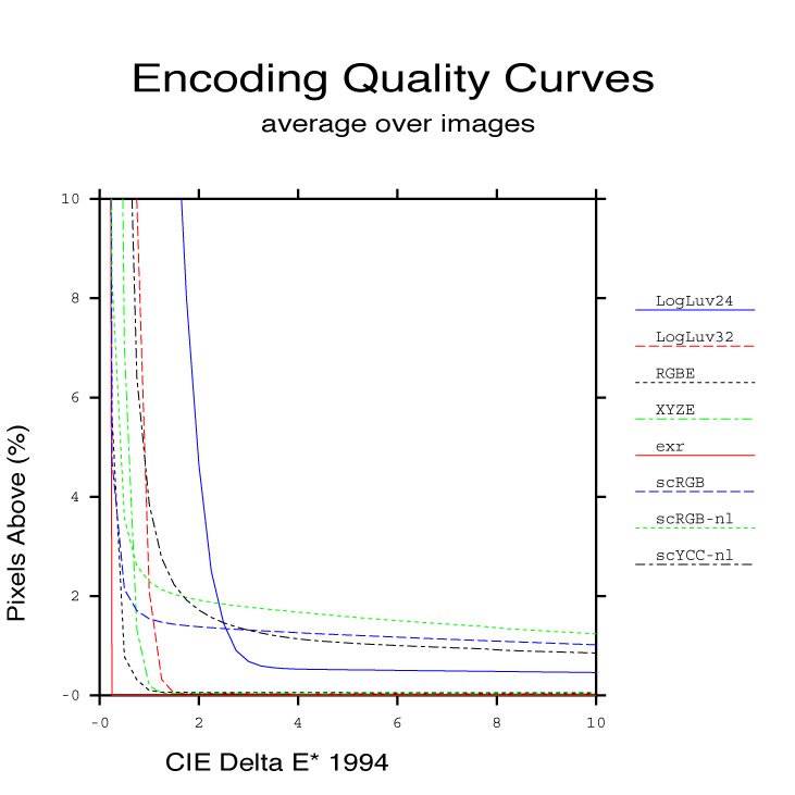
Figure 12. Summary performance of the different HDR encodings, summed over all our examples.
The biggest disappointments were the 48-bit scRGB, and the related 36-bit scRGB-nl and scYCC-nl encodings, which showed worse performance overall than their more compact predecessors, 32-bit/pixel RGBE, XYZE, and LogLuv. We should note that the scRGB format actually showed very good accuracy over the colors it was able to represent within its limited dynamic range, as demonstrated by its steep drop at the beginning. However, because many of our images would not fit within this encoding’s 3.5 orders of magnitude, the tail of the curve continues out past ∆E* values where differences are visible. Since the express purpose of an HDR format is to represent these pixels accurately, in our opinion, the scRGB, scRGB-nl, and scYCC-nl formats might be better classified as “medium dynamic range” encodings, along with the 24-bit variant of LogLuv TIFF.
Conclusion
There are many applications for high dynamic range images, and suitable formats exist in sufficient variety to support most work. The original Radiance RGBE format and its XYZE variant cover a vast dynamic range (76 orders of magnitude) with moderate accuracy (1%). The TIFF 32-bit LogLuv format covers half this range with over twice the accuracy. By comparison, the 48-bit ILM EXR format covers one quarter the LogLuv range with four times the accuracy. Each of these formats has been deployed and in use for a number of years, and they are all considered stable and reliable. The appropriate choice depends on the particular application’s need for range, accuracy, and color space flexibility.
In contrast, the new IEC standard (61966-2-2) for extended gamut color seems a poor choice for HDR image encoding. For the number of bits consumed, this format offers poor resolution and range compared to other HDR standards, and is not recommended. We hope that Microsoft will offer a revised standard for the scRGB encoding, or abandon it for an existing solution. Since there are no royalties or burdens associated with any of the established encodings, there is no particular reason to reinvent them.
There is much work to be done in the area of lossy compression formats for HDR images. This is needed especially for digital photography and digital cinema, where image bit rates are a very important practical consideration. We simply cannot afford to use 48 bits for every pixel value, or even 24 – we need to compress the data to store it and transmit it without exhausting our resources, and we are willing to suffer some data loss along the way, so long as it is kept (mostly) below the visible threshold.
We said near the beginning that pixel encodings and image wrappers are largely separable problems, but they are not completely separate. Some color encodings work better than others for compression. Many compression algorithms benefit by splitting each pixel color into a luminance channel and an opponent chroma pair. This is the idea behind the YCC encoding used in JPEG, as well as the NTSC video standard, which also downsample the chrominance channels prior to transmission. ILM has experimented with an opponent color space with downsampling, which has now been included as an experimental addition to their OpenEXR library. The LogLuv encoding is perfectly matched for this type of compression, since the CIE (u´,v´) coordinates need only an offset to be an opponent chroma pair. We hope to see such an encoding in a future version of JPEG 2000, which offers a choice of original bit lengths for its color channels.